This post is copied over (and slightly modified) from an old blog post I wrote in 2018 on wordpress. I am planning to continue a series of posts on this topic, and felt that it would be pragmatic to have the original post copied here first. I have also altered the title slightly, to reflect the theme of the series of posts more accurately

This is the first of a series of posts that take a look at the historical origins and evolution of handling software concurrency, as well as the Actor model – a mathematical model of concurrent computing put forward in the 1970s – which in recent years, has spawned the popularity of Actor based frameworks for implementing concurrent, resilient, and distributed applications.

Early origins

What we intuitively understand as concurrency became quite a complicated concept with the advent of computers. The first generation of machines were invented, and worked as ordained by the theories of computation laid down by Kurt Gödel, Alan Turing, Alonzo Church, and John von Neumann. The first generation vacuum tube behemoths ran their instructions sequentially and churned out results to humans, who for the most part, were relieved that there was a means of automating calculations and processes that they would have otherwise done manually. The second and third generation machines, with their transistors and integrated circuit innards, created large waves of change in the computing world (by and large enabling microcomputers to be inexpensive and accessible by many), but the basic software instructions and processing model remained sequential – feeding a single processor – similar to how a first generation machine would have run its instructions (to be fair, attempts at building super computers using parallelization were undertaken during this time. One such early example was the ILLIAC IV).

Mathematical models of computation

In order to lay down some foundational understanding, and to better appreciate and understand the notion of computation, we divert our attention to a quick overview of abstract models of computations known as Turing machines, Push Down Automata, and Finite State Machines. Abstract machines are the foundations of modern computers. Mathematical models of computation laid the foundations for computers and programming languages, and continue to explore the possibilities and limitations of what computers are capable of.

A finite state automata (or finite state machine – FSM) is an abstract and mathematical model of computation. Very simply put, it models an abstract machine that receives input in the form of a sequence of symbols, and can be only in one state at any given time. Changing from one state to another is known as a transition, and occurs based on the input symbol read from the sequence. From a global perspective of a FSM, the abstract machine only knows the current state it is in, and there is no concept of memory that can hold a list of previous states. Shown below is a rather contrived example of a FSM with three states – A, B, and C.

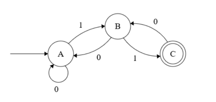
State A, where the initial arrow is pointing into, is known as the starting or initial state. State C is known as the accepting state, denoted by the double circle. The arrows between the states as well as self referencing from the state, are known as transitions. The transitions are labelled with symbols, denoting the input symbol value that will allow the transition. In the above case there are three states and a set of two input symbols {0, 1}, therefore the FSM is called a three state two symbol FSM.

Given this information, it is very easy to see what will happen if an input sequence such as 1011 is fed into the above FSM. The very initial state will be the starting state A, and from here, we read the first symbol of the input sequence 1011, which is 1. This invokes the FSM to transition state to B, and now we are in state B. The next symbol we read in is 0, which means there will be a transition from B back to A. Likewise, the next symbol is 1, which means the FSM will transition to state B, and the final symbol is 1, whereby the state will transition from B to C.

The important point to note here is, there can be arbitrarily long and complicated sequences of symbols (not limited to binary digits) being read in by the FSM, and when the final symbol of the sequence is read, the FSM could be in state C (the accepting state) or not. If it is in the accepting state after the sequence is completed, the set of symbols is known as a ‘regular language’, and the FSM is said to accept it. vice versa, a language is said to be regular, if there is some FSM that accepts it. This enables us to define that a sequence of symbols such as 1001001001001101 is a regular language to the above FSM, but 100100100100110 is not.

Definition: A regular language is a sequence of symbols that is accepted by an FSM, i.e. if it can terminate in an accepting state.

Determinism and non-determinism

FSMs can be deterministic or non-deterministic. The FSM we looked at just now is an example of a deterministic FSM, where each state can have one and only one transition for an input. In a non-deterministic FSM, an input could change the current state of the FSM by having one transition, more than on transition, or no transition at all. This brings in the notion of non-determinism to the model of FSMs. Given below is an example of a non-deterministic FSM (NFSM).

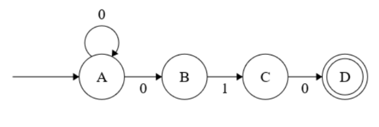
If you consider the above finite state machine, you would notice, that when in state A, if the input symbol is 0, there will be two state transitions, one to A itself, and another to B – i.e. there are two possible next states. Also, the above NFSM accepts regular languages with a sequence that ends with 010. If the state is in C, and the input symbol is 1, no state transition occurs.

There is another type of NFSM which uses what is known as ‘epsilon transitions’. In a very simple manner of looking at it, an epsilon transition means that the state change can take place without any input symbol being consumed. This will be clearer with the example of a NFSM that uses epsilon transitions as shown below.

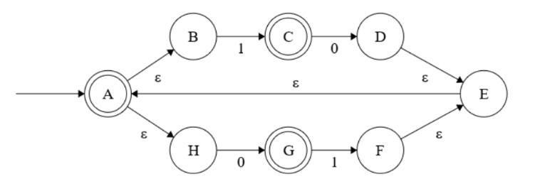
In the above NFSM, the transitions labeled with the greek letter epsilon (ε) are the epsilon transitions. State A is the starting state, as well as an accepting state. C and G are accepting states as well. Lets consider what happens when the input set (symbol sequence) consists only of the symbol 0. First, we will be in the starting state A. But as there are two epsilon transitions from A, we will go to the states pointed by these without reading in any input symbol. So we automatically go to states B and H. Now we read in the input symbol, which is 0. In this case only, state H transitions to G, and no state change takes place from B. But as the input sequence is consumed, and the NSFM terminates in an accepting state (G), we can conclude that 0 is a member of a regular language accepted by this NFSM. So is 1, 01, 10, 010, 101, 1010, etc (which can be checked against the above NFSM).

NFSMs are pretty handy when modelling reactive systems. Also, modelling a system using NFSMs is easier than using deterministic FSMs. It would seem that NFSMs are more powerful than DFSMs given the more extensive rule sets of parallel state transitions and epsilon transitions, but it can be proven that for any regular language recognized by a NFSM, there exists an equivalent DFSM that accepts that language (and vice versa). This means that there will always be an equivalent DFSM for any given NFSM. This concept allows us to design or model systems using NFSMs, and later convert it into an equivalent DFSM.

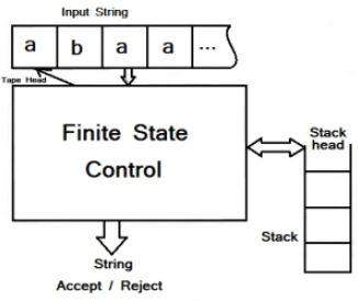
In abstract machines (such as the FSMs we saw above), the power of the machine is another way of saying it can recognize more (regular) languages. There are limitations of FSMs that are addressed by another type of abstract machine known as the pushdown automata (PDA). This can be thought of as a FSM plus a stack that can be used to store information or state in a LIFO (Last In First Out) fashion. This enables the PDA to store bit values in the stack, and come to an acceptance state only if the stack is empty once the input symbol sequence is processed. If you notice, this is a different acceptance criteria from the FSMs we saw earlier. The below image shows a snapshot of a PDA in operation.

If the power of abstract machines are determined by the languages they can recognize, then the mathematical model of computation known as Turing machines are more powerful than both FSMs and PDAs (This is another way of saying that there are sequences of input symbols that cannot be processed by FSMs or PDAs, but which are accepted by Turing machines).

Turing machines

Alan Turing published an article in 1936 titled ‘On Computable Numbers, with an Application to the Entscheidungsproblem‘, in which he first described Turing machines. A Turing machine can be thought of as a FSM with an infinite supply of a tape medium that it can read from and write to. Basically, the Turing machine reads a symbol from the tape which serves as the input symbol, and based on this input symbol, either writes a symbol to the tape, moves the tape left or right by one cell (a cell being one read/write unit of the tape which can contain a symbol), or transition to a new state. This seems a simple and basic way of operation, but Turing machines are powerful because given any algorithm, we can construct a Turing machine that can simulate that algorithm. Also, more interestingly, Turing machines have the innate ability to halt or stop, which gives rise to the halting problem.

You can find an online Turing machine simulator at this link if you would like to experiment with Turing machines (I would suggest going through the tutorials in the simulator, and then trying out with the ‘even number of zeros‘ example which is simple yet explains the fundamentals). Also, this video contains one of the best and shortest explanations of Turing machines I have seen yet.

In modelling computations and abstract machines, Turing machines are the most powerful abstraction we have today, and all out modern computers, program code, and algorithms, are based on it. The reason it is powerful is, anything that a Turing machine can simulate, can be constructed physically in the world today. But something that has no Turing equivalent system, cannot be constructed in reality (i.e. we have never come up with a way of doing computations or any mathematical model, that can do more than what a Turing machine can do – this is why for example, we do not have any system today which can solve the halting problem). In this sense, Turing machines are at the forefront of what is computationally feasible.

The next post in this series will explore the early mathematical models of concurrency and Dijkstra’s 1965 paper which addressed concurrency control for the very first time and gave rise to the dining philosophers metaphor. We will also look at how Carl Hewitt’s claim that logical (mathematical) deduction could not carry out concurrent computation due to indeterminacy, laid the foundations for the Actor model.